veri-nn implementation
Motivation
You might ask: why would anybody ever build a neural network in Verilog? There are countless high-level implementations, and dealing with transistors is not only a complete waste of time, but it sounds like a complete head-banging idea, considering that a small mistake could lead to hours of debugging. There really is no argument from me on that, and you are completely right. My main driving motivation, outside of simply technical pursuit, was to appreciate why we have high-level implementations for a lot of tasks today. In other words, why do people program in C instead of Assembly, and Python instead of C? Outside of painstakingly difficult Verilog code to write, I found this project very fun!
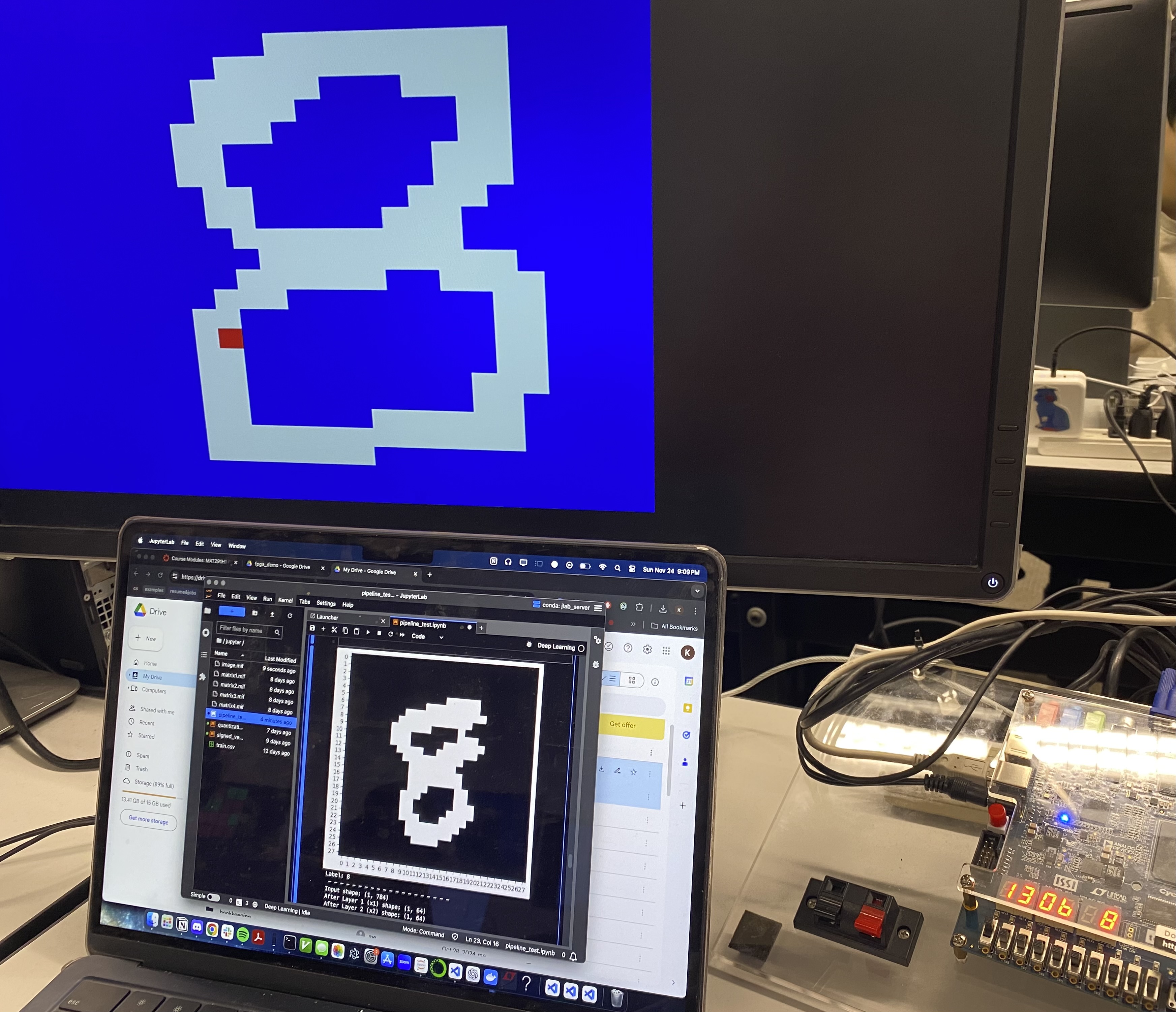
Since the neural net is quite literally embedded into the FPGA through means of a compiled circuit, there are no overheads that you might have while training in Python and PyTorch, which may be due to operating system scheduling or file reading. What makes this project very interesting is that you can actively see how the imported neural net classifies the drawn digit as the user is drawing it, which was very cool to show some niche cases where you could draw a 0, and then draw a line through the middle, making it an 8, and then the classification mechanism (HEX0), displaying the updated prediction.
Challenges
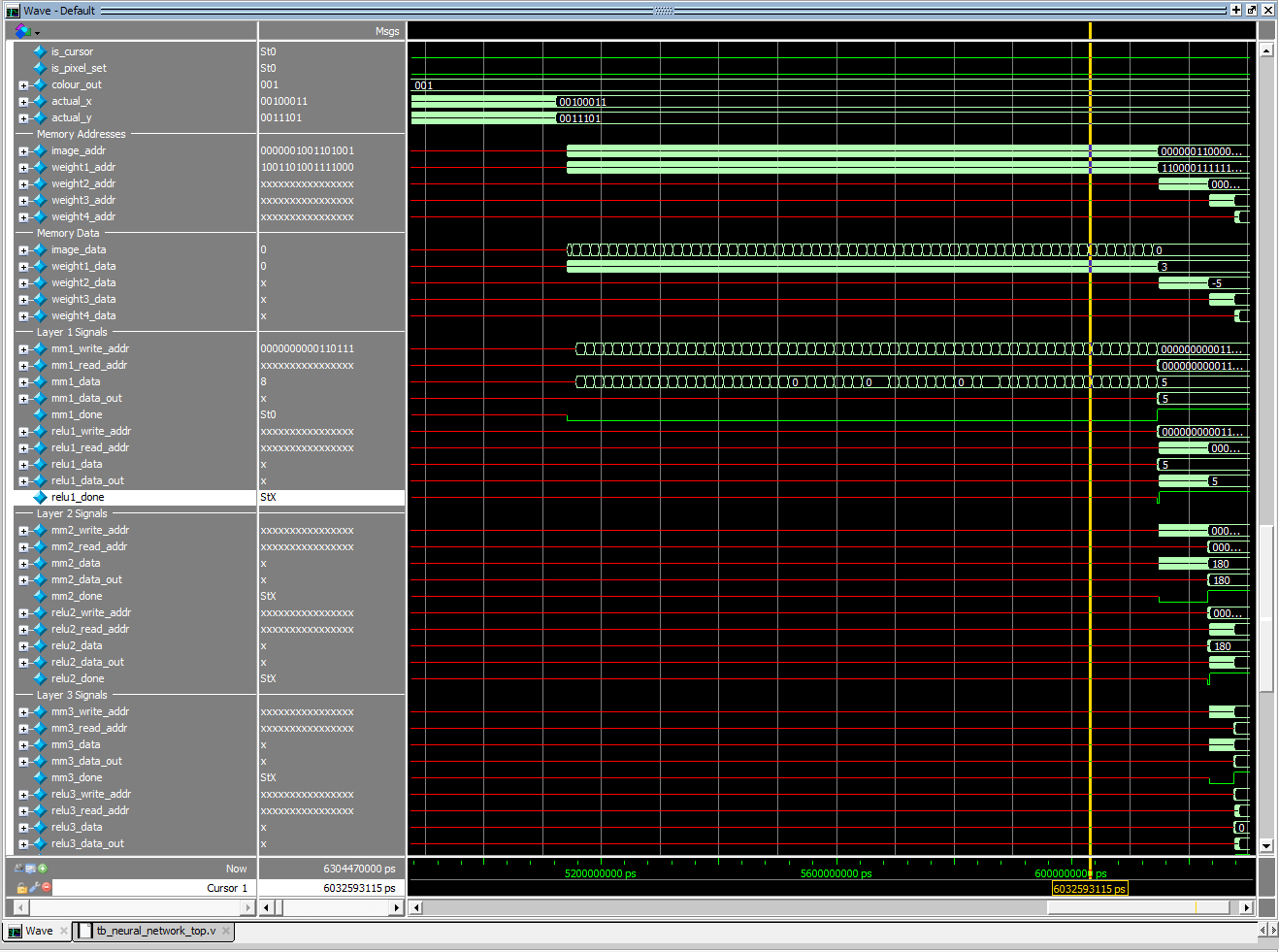
There were several challenges and solutions that I encountered while debugging, outside of boring VGA and keyboard integration. The first was the matrix multiply module, which required precise timing and constraints to Verilog’s variables. This module itself is an FSM that transitions states from starting computation, to performing computation, to finishing computation (the entire design is an FSM in an FSM, yes). To avoid complicated circuit implementations with prefetching data and all sorts of latency issues (clock skew, data delay, clock delay, and other FPGA microparameters), I added a simple if statement that waits for data to arrive before computing an accumulated dot product. Although this may not be necessary since on-chip memory is available on the same clock cycle, this allowed for there to be zero chance of timing issues in the design, which may be caused by synchronization or setup of the values (start of each dot product calculation).
This design does add a lot of overhead, since there are extra clock cycles performed for every dot product calculation. Accuracy and correctness was one of my most important design considerations, since a single race condition would lead to the implementation not working (had to debug for a long time to figure out why my calculations showed up as ‘X’ on ModelSim). Regular Verilog does not allow you to pass signals representing multi-dimensional arrays to different modules. To solve this, I computed accumulated dot products by representing each 1D matrix as a 2D matrix and using integer division as well as modulo operations to calculate them. There are many articles on this implementation, and a good one is here.
int row = index / COLS; // Calculate row using integer division
int col = index % COLS; // Calculate column using modulo
// Main FSM with enhanced memory access debugging
always @(posedge clk) begin
    case (current_state)
        IDLE: begin
            if (start) begin
                $display("\nTime=%0t | Matrix Multiplication Starting", $time);
                $display("Matrix Dimensions: M=%0d, N=%0d, K=%0d", m, n, k);
                $display("Total input matrix size: %0d", m * k);
                $display("Total weight matrix size: %0d", k * n);
                i <= 0;
                j <= 0;
                p <= 0;
                temp_sum <= 32'h0;
                done <= 0;
                final_store_done <= 0;
                last_calc_done <= 0;
                write_enable <= 0;
                wait_cycle <= 1;
                first_mult <= 1;
                input_addr <= 0;
                weight_addr <= 0;
            end
        end

        COMPUTE: begin
            write_enable <= 0;

            if (wait_cycle) begin
                wait_cycle <= 0;
            end else if (!final_store_done) begin
                if (first_mult) begin
                    temp_sum <= input_data * weight_data;
                    first_mult <= 0;
                end else begin
                    temp_sum <= temp_sum + (input_data * weight_data);
                end

                if (p == k-1) begin
                    output_addr <= i * n + j;
                    output_data <= temp_sum + (input_data * weight_data);
                    write_enable <= 1;
                    if (i == m-1 && j == n-1) begin
                        final_store_done <= 1;
                        last_calc_done <= 1;
                    end else begin
                        if (j == n-1) begin
                            i <= i + 1;
                            j <= 0;
                        end else begin
                            j <= j + 1;
                        end
                        p <= 0;
                        temp_sum <= 0;
                        wait_cycle <= 1;
                        first_mult <= 1;
                        input_addr <= (j == n-1) ? (i + 1) * k : i * k;
                        weight_addr <= (j == n-1) ? 0 : (j + 1);
                    end
                end else begin
                    p <= p + 1;
                    input_addr <= i * k + p + 1;
                    weight_addr <= (p + 1) * n + j;
                end
            end
        end

        FINISH: begin
            done <= 1;
            write_enable <= 0;
        end
    endcase
end
Another major challenge of this design was the 0.537 MB memory constraint. There are 440 M10K blocks of on-chip memory, that can each store 10,240 bits. This totals out to 4,505,600 bits, which is where I got 0.537 MB from. To meet this constraint, I had to carefully calculate the total memory of my neural network to stay under this, and also leave a small amount of room for any additional signals from all other parts of my design, including the main FSM, the VGA, and the keyboard modules. I decided on the architecture (784, 64), (128, 64), (64, 32), (32, 10), with ReLU activations in between. The total calculations are summed up here for all layers, and one 1 x dim for the input, as well as 2 x dim for the output of each matrix multiplication, and each ReLU activation. I may have messed up these calculations, so please correct me if I do (multiplying 32 by the total # of bits for each storage element since my precision is int32).
32 (1 x 784 + 784 x 64 + 2 x 64 + 64 x 32 + 2 x 32 + 32 x 10 + 2 x 10)
This totals out to 1,713,280 bits, which is far under my constraint! Future implementations could try expanding this to potentially allow for higher accuracy model imports. What could really help is changing the first layer to transform an image to a (1, 128) tensor instead of a (1, 64) tensor, which would still be within constraints.
Leading on from this, another issue was training my neural network using integer weights. Although PyTorch has libraries for quantization, I noticed that my initial use of a quantization pipeline would not be able to converge to a desirable accuracy. What worked out was implementing a “gradual scaling” that would scale the weights over each epoch, instead of all at once, completely truncating the fp32 values to int32.
# Entry point in training loop that scales our weights
def gradual_scale_weights(model, initial_target_min, initial_target_max, final_target_min, final_target_max, step_size, epoch, max_epochs):
    # Gradually scale the weights of each layer after each epoch.
    # Compute the scaling range for this epoch based on the progress in training
    scale_min = initial_target_min + (final_target_min - initial_target_min) * (epoch / max_epochs)
    scale_max = initial_target_max + (final_target_max - initial_target_max) * (epoch / max_epochs)
    # Apply gradual scaling to each layer
    model.scale_weights(target_min=int(scale_min), target_max=int(scale_max))
class ScalableLinear(nn.Module):
    def __init__(self, in_features, out_features):
        super().__init__()
        self.weight = nn.Parameter(torch.randn(in_features, out_features, dtype=torch.float32))  # Initialize weights

    def forward(self, x):
        return x @ self.weight

    def scale_weights(self, target_min, target_max):
        with torch.no_grad():
            # Get the min and max values of the layer's weights
            weight_min = self.weight.min()
            weight_max = self.weight.max()

            # Compute scaling factor
            scale = (target_max - target_min) / (weight_max - weight_min)
            zero_point = target_min - weight_min * scale

            # Apply scaling to weights
            quantized_weights = torch.round(self.weight * scale + zero_point)

            # Clip to the target range (make sure no value goes outside the desired range)
            quantized_weights = torch.clamp(quantized_weights, target_min, target_max)

            # Update weights directly
            self.weight.data = quantized_weights
The original approach, to scale weights, was way too drastic, and the model was unable to converge and deal with the loss in precision all at once due to its small size, and reliance on small values initially.
Through playing with combinations of hyperparameters, I was finally able to get a max validation accuracy of about 80%! This can be improved by making the neural net have larger weights (within the constraints of the on-chip memory). What was interesting was that with the same hyperparameter setup, a single sequence run could randomly give high accuracy over a reasonable number of epochs, while several other sequence runs would never train past 50% training accuracy. This may be because of the fact that since the neural network’s weights are randomized based on a Xavier initialization—Xavier Initialization—the weight matrices at initialization are evenly distributed. Due to the small size of the network, as well as the loss in precision, randomness played a key factor in helping me train the network!
My final precision was 32-bit unsigned, which can allow for numbers ranging from -2^31 to 2^31 - 1. Theoretically, the user could cause integer overflow, however, the chance of this is really low, since my input image is a bitmap of 0s and 1s, and the weights are all scaled between -31 and 32. It would be very hard for an accumulated dot product to produce a number greater than 2^31 (2147483648)!
Another small challenge I had was race conditions due to my memory matrix interface. Specifically, the interface looked like this:
mm1_memory mm1_mem(
    .clk(clk),
    .write_addr(mm1_write_addr),
    .read_addr(mm1_read_addr),
    .data_in(mm1_data),
    .write_enable(write_mm1),
    .data_out(mm1_data_out)
);
I used a “getters” and “setters” approach in my implementation as read_addr and write_addr. This is a concept usually taught for C++, and I initially thought it was useless. However, it ended up helping me solve the race condition issues that I had initially had, due to driving an address signal somewhere (this idea really came in clutch on this project!).
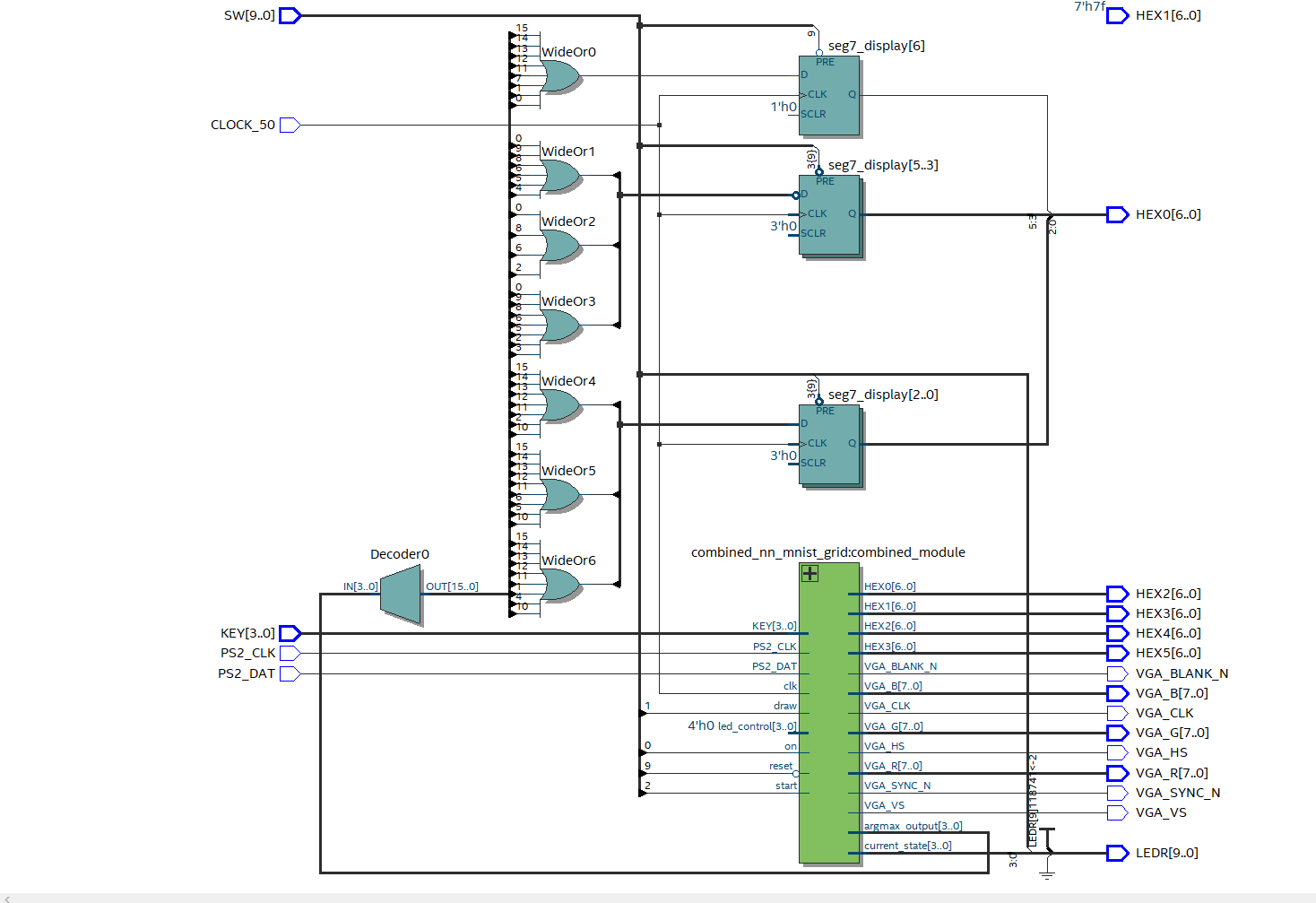
Finally, the last issue I had was the Verilog syntax of output vs input signals declared in module instantiations. As shown above, I used addresses and moved them around to access the internal memory variables inside the memory module instantiations. Any modules such as my matrix multiplication module and ReLU module should get passed the corresponding address for accessing the memory variables. If we imagine module instantiations as a tree (relation defined by parent that defines the child module), although Verilog is NOT a programming language as heavily emphasized by one of my professors, it is helpful to view it through this perspective, since any module that has the corresponding addresses passed in (accessing the internal memory variables inside the memory module instantiation) must have the same parent module. In other words, there is no clever way to pass the addresses in and out of modules, and this is the only way. One thing that was really hard to debug was the fact that ModelSim would allow a smart manipulation of output and input variable pipelines, but it would not work on the FPGA (although this might not be the correct conclusion, this realization was the reason I was able to finish the project).
Codebase Overview
I have gone over many of the most important features of the codebase, but there are a few more to specifically cover. The neural network can be interpreted as an FSM. However, instead of an FSM that changes state based on the clock, the FSM changes states based on asserted done signals. This implementation allows for an easy interface, that can be expanded and reduced as desired.
// State machine control logic
always @(posedge clk) begin
    start_mm1 = 0;
    start_relu1 = 0;
    start_mm2 = 0;
    start_relu2 = 0;
    start_mm3 = 0;
    start_relu3 = 0;
    start_mm4 = 0;
    start_argmax = 0;

    case (current_state)
        IDLE: begin
            if (start) next_state = LAYER1_MM;
            else next_state = IDLE;
            start_mm1 = start;
        end

        LAYER1_MM: begin
            if (mm1_done) begin
                next_state = LAYER1_RELU;
                start_relu1 = 1;
            end else begin
                next_state = LAYER1_MM;
            end
        end

        LAYER1_RELU: begin
            if (relu1_done) begin
                next_state = LAYER2_MM;
                start_mm2 = 1;
            end else begin
                next_state = LAYER1_RELU;
            end
        end

        LAYER2_MM: begin
            if (mm2_done) begin
                next_state = LAYER2_RELU;
                start_relu2 = 1;
            end else begin
                next_state = LAYER2_MM;
            end
        end

        LAYER2_RELU: begin
            if (relu2_done) begin
                next_state = LAYER3_MM;
                start_mm3 = 1;
            end else begin
                next_state = LAYER2_RELU;
            end
        end

        LAYER3_MM: begin
            if (mm3_done) begin
                next_state = LAYER3_RELU;
                start_relu3 = 1;
            end else begin
                next_state = LAYER3_MM;
            end
        end

        LAYER3_RELU: begin
            if (relu3_done) begin
                next_state = LAYER4_MM;
                start_mm4 = 1;
            end else begin
                next_state = LAYER3_RELU;
            end
        end

        LAYER4_MM: begin
            if (mm4_done) begin
                next_state = ARGMAX;
                start_argmax = 1;
            end else begin
                next_state = LAYER4_MM;
            end
        end

        ARGMAX: begin
            if (argmax_done) next_state = DONE;
            else next_state = ARGMAX;
        end

        DONE: begin
            next_state = IDLE;
        end

        default: begin
            next_state = IDLE;
        end
    endcase
end

// Output assignment
assign done = (current_state == DONE);
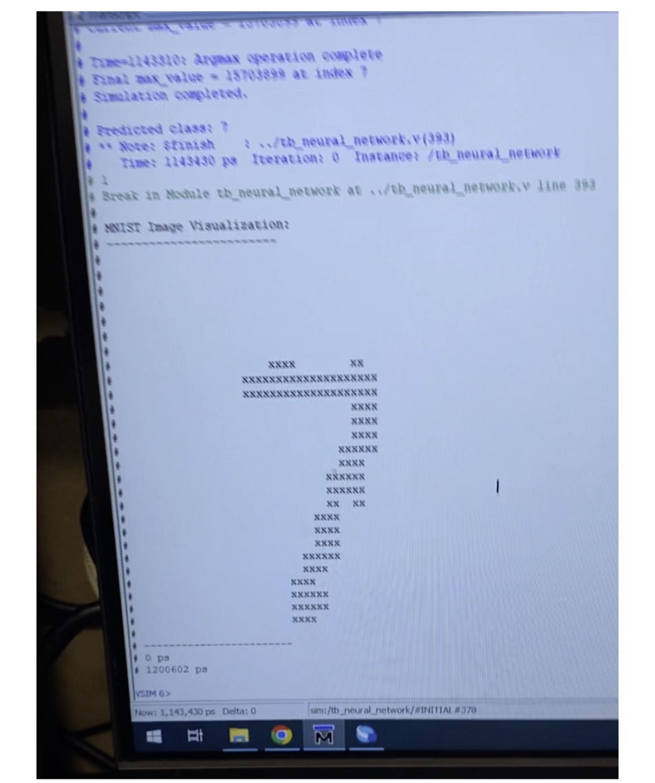
This covers nearly the entire codebase! The rest is just initializing .mif (memory initialized files) files directly importing from trained weight matrices. Another part this is not covered explicitly is the ReLU function, which just involves a similar FSM, but just reading the signed bit (last bit on the left), and then zeroing out the number if it is a 1 (same thing as ReLU). I also left the argmax function out, which is a similar element by element comparison, that saves the index of the highest activation (the output prediction).
The final product looks like this! Doesn’t look too bad for a collection of transistors.